Robust Cognitive–Flexible Filtering
under Noisy Innovation Scores
A margin that knows when to trust itself — and when the noise has changed.
Detect structural mismatch, Switch only when evidence is clear, and Adapt the margin online as the noise itself changes.
Belief \(\mathfrak{B}_t\) → Batch-split scores → Adaptive margin \(\delta_t\) → Structure \(s_{t+1}\) → Belief \(\mathfrak{B}_{t+1}\)
The margin tracks the score noise online, at zero extra Monte Carlo cost.
Graphical Abstract
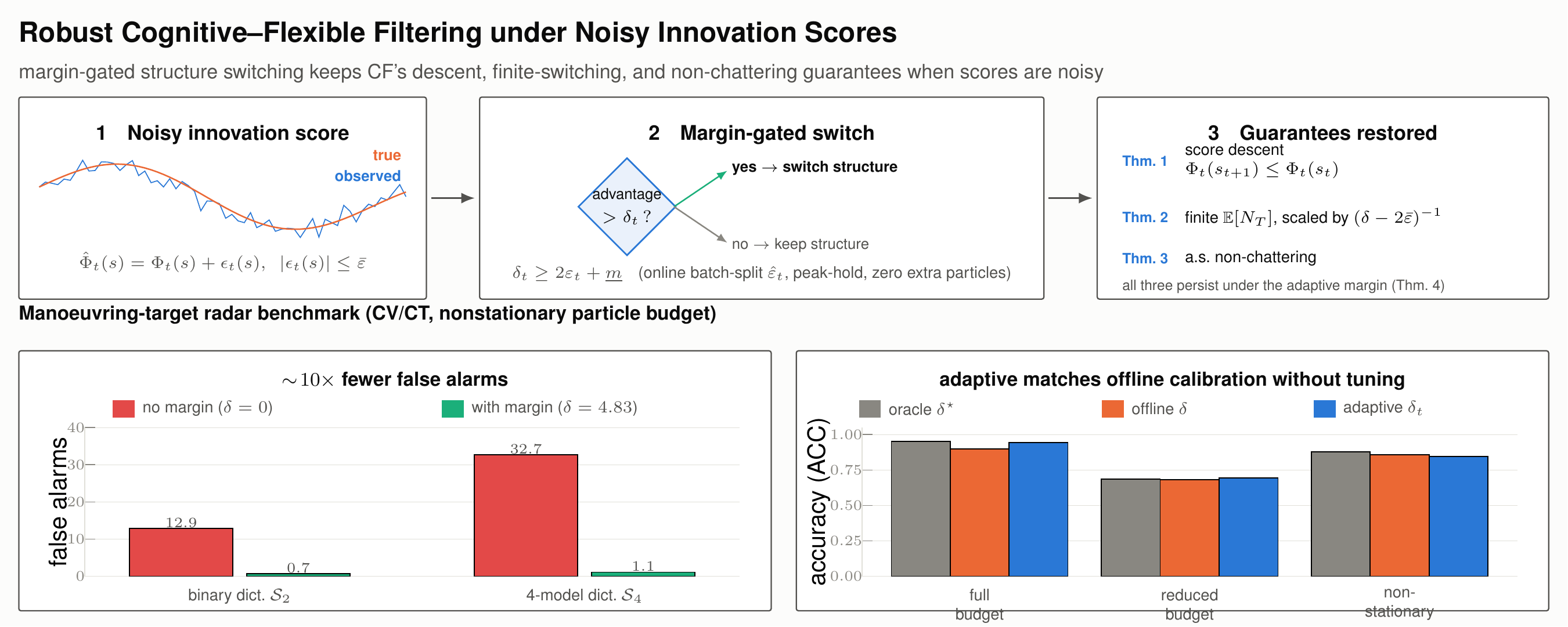
Adaptive Margin Architecture: A batch-split estimator extracts score noise variance \(\hat{\varepsilon}_t\) from existing particles with zero overhead. This dynamically scales an adaptive margin \(\delta_t\), structurally preventing noise-induced spurious switching while rigorously preserving descent and finite-switching guarantees under nonstationary regimes.
What Is the Problem?
Cognitive Flexibility (CF) selects, at each step, the latent structure \(s\in\mathcal{S}\) minimising an innovation-based predictive score \(\Phi_t(s):=-\log\ell_{\theta,s}(y_{t+1}|\mathfrak{B}_t,u_t)\), leaving the underlying filter recursion intact. Under exact scores, three guarantees hold: descent in expectation, finite switching, and non-chattering.
In practice scores are estimated by a particle filter and carry additive perturbations \(\epsilon_t(s)\) with \(\mathbb{E}[\epsilon_t(s)\mid\mathcal{I}_t]=0\) and \(|\epsilon_t(s)|\leq\bar{\varepsilon}\) a.s. Unprotected score minimisation is vulnerable to spurious switching — and any margin \(\delta\) calibrated to suppress it must, in a nonstationary setting, be calibrated against a noise level that keeps changing. This letter asks — and answers — does the theory survive noisy scores, and can the margin itself be found online, without a stationary calibration window?
⚙ The Margin-Based Rule
We introduce the margin-based switching rule:
\[ s_{t+1} = \begin{cases} \hat{s}_t, & \hat{\Phi}_t(s_t) - \hat{\Phi}_t(\hat{s}_t) > \delta_t, \\ s_t, & \text{otherwise,} \end{cases} \quad \hat{s}_t\in\arg\min_{s}\hat{\Phi}_t(s), \]
with \(\delta_t\ge2\varepsilon_t+\underline{m}\) for a deterministic floor \(\underline{m}>0\). The static case \(\delta\equiv\text{const}>2\bar{\varepsilon}\) is recovered exactly as a special case, and restores all three noiseless-style guarantees with no change to the filter recursion.
📐 Main Theoretical Guarantees
- Theorem 1 (Descent): \(\mathbb{E}[\Phi_t(s_{t+1})\mid\mathcal{I}_t] \leq\mathbb{E}[\Phi_t(s_t)\mid\mathcal{I}_t]\) for all \(t\geq0\) — the expected score never increases after a switch, regardless of noise.
- Theorem 2 (Finite expected switching): \[ \mathbb{E}[N_T]\leq\frac{1}{\delta-2\bar{\varepsilon}} \sum_{t=0}^{T-1} \mathbb{E}\!\left[\Phi_t(s_t)-\min_s\Phi_t(s)\right] \]
- Theorem 3 (Non-chattering): if \(\limsup_{t\to\infty}[\Phi_t(s_t)-\min_s\Phi_t(s)] <\delta-2\bar{\varepsilon}\) a.s., switching stops a.s.
- Theorem 4 (adaptive margin, new): replacing \(\bar{\varepsilon},\delta\) by \(\mathcal{I}_t\)-adapted \(\varepsilon_t,\delta_t\), all three guarantees persist whenever the effective margin \(\delta_t-2\varepsilon_t\) stays above a floor. The operative quantity was never \(\delta\) itself.
⚡ Zero-Overhead Online Calibration
A sliding window across time cannot estimate \(\varepsilon_t\) safely: its variability mixes genuine dynamic variation of the state with Monte Carlo error, and so overestimates the noise exactly when the system is most nonstationary. We instead exploit variability within a single time step: partition the existing \(N_p\) particles into \(B\) independently resampled batches. All batches see the same belief and observation, so their spread is pure Monte Carlo noise, invariant to the dynamics.
\[ \hat{\varepsilon}_t=\frac{\kappa}{\sqrt{B}} \max_{s\in\mathcal{S}}\operatorname{std}_{b\leq B} \{\hat{\Phi}_t^{(b)}(s)\}, \qquad \varepsilon^{\mathrm{env}}_t=\max\{\hat{\varepsilon}_t,\, \lambda\,\varepsilon^{\mathrm{env}}_{t-1}\}, \qquad \delta_t=\max\{(2+\eta)\varepsilon^{\mathrm{env}}_{t-1}, \delta_{\min}\}. \]
The peak-hold envelope rises immediately when the noise grows and relaxes only geometrically when it falls — the correct asymmetry for a quantity that must upper-bound a perturbation. Because the batches partition an unchanged particle budget, the scheme adds zero extra Monte Carlo cost: only \(O(BK)\) scalar operations per step.
Numerical Experiments
We validate on the Li–Jilkov constant-velocity / coordinated-turn (CV/CT) manoeuvring target benchmark, a standard testbed for multiple-model tracking — not a synthetic scalar model. The target state is \(x_t=[p_x,\dot{p}_x,p_y,\dot{p}_y]^\top\in\mathbb{R}^4\), where \(p_x,p_y\) are position components in the horizontal plane and \(\dot{p}_x,\dot{p}_y\) the corresponding velocities, following \(x_{t+1}=F_tx_t+w_t\), \(w_t\sim\mathcal{N}(0,Q)\). The true structure switches as CV~(\(t{<}30\)) \(\to\) CT~(\(30{\leq}t{<}70\)) \(\to\) CV~(\(t{\geq}70\)).
Transition matrices (omitted from the letter for space; \(\Delta t\) is the sampling interval and \(\omega\) the turn rate):
\[ F_\mathrm{CV} = \begin{bmatrix} 1 & \Delta t & 0 & 0\\ 0 & 1 & 0 & 0\\ 0 & 0 & 1 & \Delta t\\ 0 & 0 & 0 & 1 \end{bmatrix} \]
\[ F_\mathrm{CT} = \begin{bmatrix} 1 & \frac{\sin\omega\Delta t}{\omega} & 0 & -\frac{1-\cos\omega\Delta t}{\omega}\\ 0 & \cos\omega\Delta t & 0 & -\sin\omega\Delta t\\ 0 & \frac{1-\cos\omega\Delta t}{\omega} & 1 & \frac{\sin\omega\Delta t}{\omega}\\ 0 & \sin\omega\Delta t & 0 & \cos\omega\Delta t \end{bmatrix} \]
CT reduces to CV as \(\omega\to0\) (L’H\^opital on both fractions). The near-constant-acceleration model used in the four-model dictionary shares this 4-D state space with inflated process noise rather than an augmented state.
Two candidate sets are used: the binary \(\mathcal{S}_2=\{s_\mathrm{CV},s_\mathrm{CT}\}\), and the four-model dictionary \(\mathcal{S}_4\) adding left/right coordinated turns and a near-constant-acceleration model, chosen so that several candidates stay plausible throughout the manoeuvre.
Crucially, score noise is not injected: scores are genuine particle-filter estimates, and nonstationarity is imposed physically by a particle-budget schedule — \(N_p=4000\) except \(N_p=60\) on \(t\in[40,75)\), as a radar resource manager reallocating effort across tracks would. This moves the noise scale directly: the 95th percentile of \(\hat{\varepsilon}_t\) rises from \(1.93\) to \(5.92\), a factor of \(3.07\). The schedule places the recovery transition at \(t=70\) inside the reduced-budget window, so a genuine structural change must be detected exactly when the scores are least reliable.
Table I: Switching and Detection Metrics
| Method | \(\mathcal{S}_2\) (\(K=2\)) | \(\mathcal{S}_4\) (\(K=4\)) | ||||||
|---|---|---|---|---|---|---|---|---|
| \(\mathbb{E}[N_T]\) | FA | \(D_1\) | ACC | \(\mathbb{E}[N_T]\) | FA | \(D_1\) | ACC | |
| CF without margin | 17.5 | 12.9 | 1.0 | 0.840 | 40.6 | 32.7 | 1.0 | 0.637 |
| Fixed \(\delta=4.83\) | 2.5 | 0.7 | 3.2 | 0.873 | 3.2 | 1.1 | 3.6 | 0.734 |
| Fixed \(\delta=14.81\) | 0.6 | 0.4 | 32.8 | 0.591 | 0.7 | 0.5 | 32.1 | 0.548 |
| Adaptive \(\delta_t\) | 3.9 | 1.9 | 1.4 | 0.849 | 4.3 | 2.8 | 2.0 | 0.688 |
| IMM, \(p_\mathrm{stay}=0.99\) | 3.6 | 1.5 | 1.5 | 0.897 | 7.5 | 4.6 | 1.8 | 0.723 |
\(\mathbb{E}[N_T]\): switches; FA: false alarms outside transition windows; \(D_1\): detection delay at \(t=30\); ACC: selection accuracy. \(\mathbb{E}[N_T]\) alone is misleading — the largest fixed margin minimises it purely by failing to react.
Table II: Removing the Calibration Stage
| Procedure | full budget | reduced budget | nonstationary |
|---|---|---|---|
| Oracle \(\delta^\star\) (ground truth) | 0.951 | 0.685 | 0.879 |
| Offline rule, \(\delta{=}4.83\) | 0.898 | 0.681 | 0.857 |
| Adaptive \(\delta_t\) (no tuning) | 0.943 | 0.693 | 0.847 |
| Adaptive \(-\) offline (paired, 95% CI) | \(+0.045\pm0.030\) | \(+0.012\pm0.029\) | \(-0.010\pm0.027\) |
Selection accuracy on \(\mathcal{S}_2\), \(M=50\) per point. The adaptive rule is significantly better at full budget and statistically indistinguishable from offline calibration in the other two regimes (pooled \(+0.016\pm0.017\)).
Impact and Applications
- Adaptive state estimation under sensor noise and model uncertainty
- Particle filter-based systems where score approximation errors are unavoidable
- Manoeuvring target tracking with resource-managed (time-varying) particle budgets
- Neural-network-aided filtering (KalmanNet, Split-KalmanNet, Latent-KalmanNet) where learned scores carry structured, nonstationary errors
- Supervisory control and fault detection under drifting noise levels
Reproducibility
Julia source code is publicly available:
-
radar_final_v6b_SPLrevision_2_1_IMM.jl— Li–Jilkov CV/CT benchmark, batch-split estimator, adaptive margin, three-regime sweep (Fig. 1, Tables I–II)